The Backdrop

It took humans less than a decade to reach a level of sophistication to reach a stage where with less than a couple of keystrokes on a phone one could get the most elaborate meal delivered at home. That’s the magic of the internet revolution. In recent times this trend has only gotten sharper and sharper, with the on-demand delivery space heating up, an Indian consumer can receive anything from an egg to the most lavish dinner faster than it takes to respond to a slack message.

In fact, as of 2022 you can get most things delivered under 10 minutes! The implication of this is that the customers do not need to plan anything much in advance and that the time between desire, action, and gratification has shrunk to almost zero. One such Hypothetical unicorn startup in this space is Hyper - Which started over two years ago and has seen massive growth in a short period. Hyper is known mainly for its super fast, sub-10-minute delivery of almost anything that one can think. However, In the past couple of weeks, the sentiment trends around sub-10-minute style deliveries has been sharply negative due to various factors. Especially concerned around the lack of empathy towards Hyper’s delivery partners. What was once a strength seems to be turning into pain for the company. Many are asking if we have gone too far.

Within this Hypothetical backdrop where Hyper is reevaluating its business strategy, Hyper’s engineering team set’s forth on a journey to contribute towards its initiative of bringing a bit more balance within the marketplace. This marketplace is not overly user-centric but is also fair for other stakeholders like delivery partners. Enter recommendation systems, systems that sit at the heart of how most digital marketplaces perform. Most digital economies are shaped by these systems. The scale, convenience, and speed of marketplaces like Hyper are enabled by recommendation systems and search engines. Hence, what these systems optimize for and how they behave are of critical importance. Within a marketplace, multiple factors come into play, and the success of any given marketplace is closely tied to how you match, cater & satisfy the requirements of all the stakeholders like the consumers, suppliers, and more. In a series of articles, let’s dive deeper into how these systems are designed, optimized and explore the inner workings and learn how some parts of these systems are built in practice.

But first, let’s establish a couple of definitions, terms & concepts.

🧵 Marketplace, marketplace differentiators & superstar economics

Marketplace: An intermediary that helps facilitate economic interaction between two or more sets of agents, these have existed since time immemorial as local markets to shopping malls to modern digital experiences like amazon, Flipkart, Swiggy, Instacart, etc - in fact, they are pretty much everywhere.
Differentiating factors of a marketplace: Marketplaces come in various shapes and sizes, but at a high level they can be differentiated based on Need/Customer coverage (horizontal vs vertical), Participant type (b2b vs b2c), Type of offering (service, goods, information, etc). They can also be differentiated based on control and functionality styles (open, closed, focused, censored, etc), management approach (unmanaged, lite, or fully managed) & lastly their transaction regularity (one-off & repeat transactions).
Superstar economics: The Phenomenon of superstars, wherein a relatively small number of people earn enormous amounts of money or value of some form and dominate the activities in which they engage.

Introduction

At the core of any recommendation system, there would be something like a collaborative filtering model (matrix factorization or tensor factorization), latent variable model, neural embeddings-based model, or Neural Collaborative filtering models, and these systems would come in one of these variants - Short vs Long term recommendations, cold start & cohort-based, Multi view and multi-interest models or multi-task recommendations. The most common trend in all these systems usually would be that they all are focused on delivering single user-centric recommendations. These systems were designed to address concerns around user needs, behavior, interests, interactions & personalization. Further, they are measured on user engagement-oriented metrics.

But, caring only about a single user type, might not yield the most optimal outcome especially when there are many stakeholders involved within a platform - aka recommendation systems within a marketplace-type setting could not be designed with a single entity in mind. This is where the need for a recommendation system that caters to different stakeholders with different sets of interests arises.

Hence, Recommendations in marketplaces are multi-sided. Equipped to cater not just to a single user’s (aka buyer) needs, but also the supplier’s needs & most often they also have to consider platform economics within the play. Such a system is usually designed with many objectives in mind - some of these objectives are User expectations, user understanding, supplier exposure, supplier goals, platform objectives, and long-term value.

Now let’s further look into these different stakeholders, their objectives & the interplay between these objectives that usually arise within this ecosystem.

Stakeholders, Objectives & the Objective interplay

In a multi-sided system with multiple objectives often the objectives interact and behave in different manners. At a high level, you could categorize the different types of these interplay as follows:

Correlated : Optimising for one objective helps the other.
Neutral: Optimising for one does not impact the other
Anti Correlated: Optimising for one hurts the other

Consider the example of our Hypothetical on-demand delivery startup Hyper, which is a three-sided marketplace - i.e it has three sets of stakeholders with different motivations & objectives.

Stakeholder	Needs/Motivations	Potential Objectives
End User	Wants to order something from local partner shops.	Quick delivery Best price Reliable merchants Fresh items
Merchants	Provide online visibility and find customers.	Matching quality Exposure Minimise wastage
Delivery Partners	Earn a stable livelihood.	Regularity in jobs Earnings per partner Efficient drop location planning

As we see above each entity has a unique set of potential objectives one could optimise the recommendation system for & this has to be done in a deliberate and careful way or it might result in undesired outcomes.

🧵 Superstar economics and towards a fair marketplace

Researchers from Microsoft & Spotify found out that:

Recommendation systems in general suffer from what is called as an inherent problem of “superstar economics”: rankings have a top and a tail end, not just for popularity, but also for relevance. In an attempt to maximize user satisfaction, recommender system optimize for relevance. This inadvertently leads to lock-in of popular and relevant suppliers, especially for users who want to minimize the effort required to interact with the system. A major side-effect of the superstar economics is the impedance to suppliers on the tail-end of the spectrum, who struggle to attract consumers, given the low exposure, and thus, are not satisfied with the marketplace. Indeed, to continue to attract more suppliers to the platform, marketplaces face an interesting problem of optimizing their models for supplier exposure, and visibility. Indeed, the suppliers (e.g. retailers, artists) would want a fair opportunity to be presented to the users.

In short, what a system optimizes for is super important & in general, it needs to look for a balance while optimizing for various objectives.

Before we proceed further on how to optimize for multiple objectives let us quickly revisit and see how most modern recommendation systems are built. Also, let’s do a quick recap of how one builds a ranking model (aka Learning to rank) & some important metrics used for measuring these systems.

A Quick Recap on modern recsys

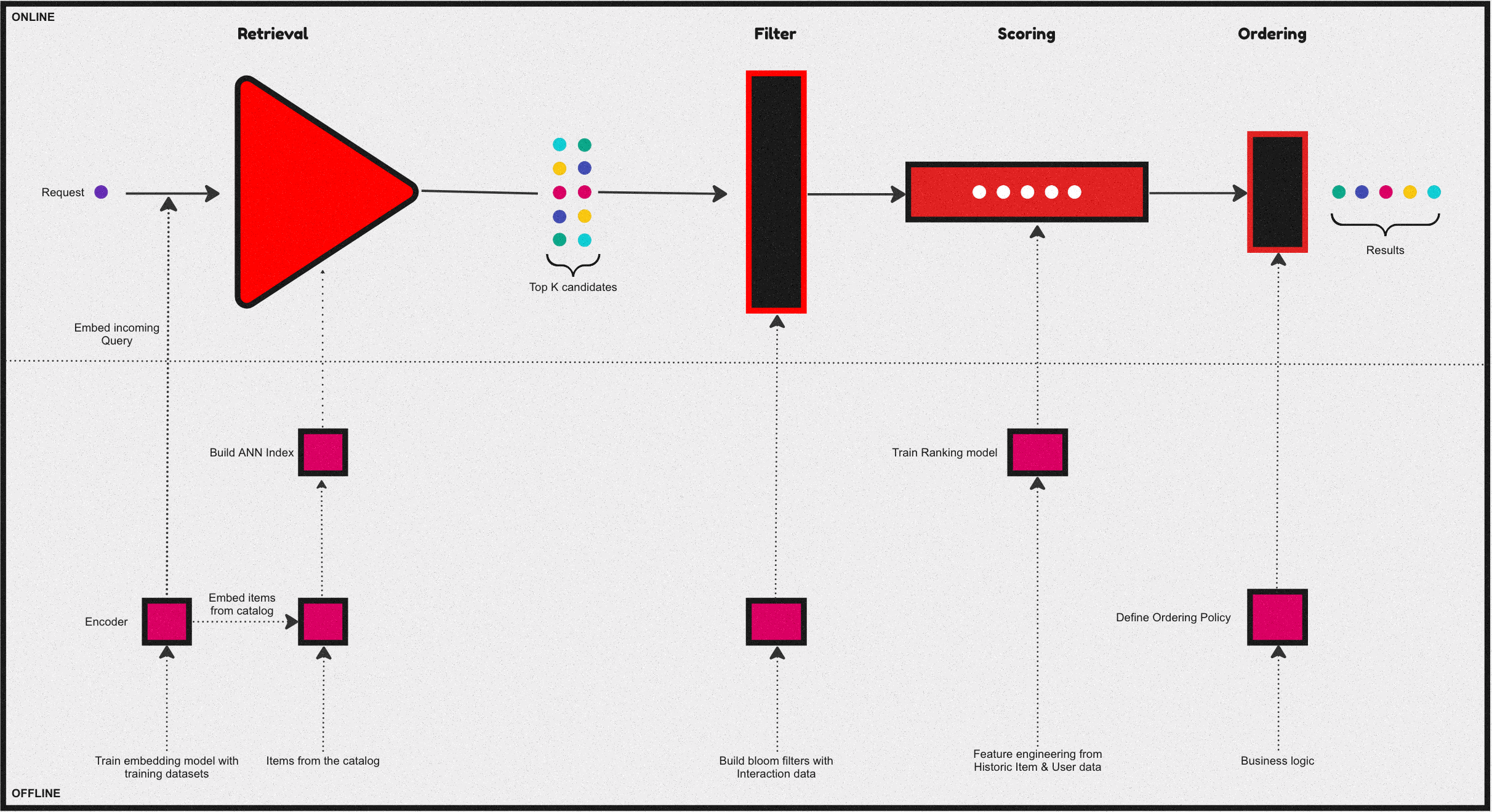
Over the past few years, a common and central design pattern has emerged around how most industrial recommendation systems are designed. If one were to summarise this design pattern, it would appear as described in the above figure - consisting of 4 stages. Let us take a brief look at the functionality of these four stages:

Candidate retrieval

The Retrieval & filtering stages usually are collectively referred to as candidate generation. A fast but coarse step which narrows down the search space of items from millions of candidates for a given query to something in the order of 100s.

Often this is achieved by an initial retrieval with some form of matching between the query and the catalog.Usually, via an ANN, Graph-based approach, or some form of a decision tree. Followed by a filtering stage, where invalid candidates are removed from the initial retrieval before passing on to the next stages.

Ranking

At this phase, we further narrow the initial set of items into a much smaller list to be presented to the user. Which is a slow but more precise operation - this stage is usually modeled as an LTR or a classification task. Further, sometimes it’s followed by an ordering stage which handles various business logic to reorder/sort the final list of items. Some common examples of this business logic include: organizing recommendations to fit genre distributions in streaming services or promoting specific segments of sellers as in the case of e-commerce.

📝 Suggested reading

Most Production recommendation systems are indeed complex in nature, but the above pattern which was conceptulised at Nvidea by @Even_Oldridge & @karlhigley sort of provides a good overview of how these systems are designed & to read a bit more on this, refer to Recommender Systems not just recommender models article & also read system-design-for-discovery from @eugeneyan where he summarises this design pattern in depth and points to multiple examples from industry that follow this pattern.

A Quick Recap on Learning to Rank

Learning to rank (LTR) refers to a class of ML techniques for training a model to solve the task of ranking a set of items. Usually, this is formulated as a supervised or sometimes semi-supervised task.

Generally, this means we try to learn a function \(f(q, D)\) given a query \(q\) & a list of documents \(D\) to predict the order/rank of the documents within this list. Depending on how the loss function is formulated in the underlying task, any LTR algorithm can be classified into 3 distinct categories:

Pointwise method
Pairwise method
Listwise method

Ranking Task

Given a query \(q\), and a set of \(n\) documents \(D=d_1,d_2,...,dn\), we’d like to learn a function \(f\) such that \(f(q, D)\) will predict the relevance of any given document associated with a query.

Pointwise method

In pointwise method, the above ranking task is re-formulated as a standard classification/regression task. The function to be learned \(f(q, D)\) is simplified as \(f(q, d_i)\) i.e the relevance of each document given a query is scored independently.

For instance, if we have two queries associated with 2 and 3 resulting matched documents:

\(q_1 \to d_1, d_2\)
\(q_2 \to d_3, d_4, d_5\)

Then the training data \(x_i\) in a pointwise method will essentially be every query-document pair as follows:

\(x_1 : q_1, d_1\)
\(x_2 : q_1, d_2\)
\(x_3 : q_2, d_3\)
\(x_4 : q_2, d_4\)
\(x_5 : q_2, d_5\)

Since each document is scored independently with the absolute relevance as the target label, the task is no different from any standard classification or regression task. As such any standard ml algorithms can be leveraged in this setting.

Pairwise method

In pairwise method, the goal is to learn a pointwise scoring function \(f(q, d_i)\) similar to a pointwise formulation. However, the key difference arises in how the training data is consructed - where we take pairs of documents within the same query as training samples.

\(x_1 \to q_1, (d_1, d_2)\)
\(x_2 \to q_1, (d_3, d_4)\)
\(x_3 \to q_1, (d_3, d_5)\)
\(x_4 \to q_1, (d_4, d_5)\)

In this setting, a new set of pairwise binary labels are derived, by comapring the individual relevance score in each pair. For example, given the first query \(q_1\), if \(y_1==\) (i.e.. an irrelevant document) for \(d_1\) & \(y_2=3\) (i.e.. a Highly relevant document) for \(d_2\) then we can create a new label \(y_1<y_2\) for the pair of docs \((d_1, d_2)\) - by doing so we have essentially converted this back to a binary classification task again.

Now in order to learn the function \(f(q, d_i)\) which is still pointwise, but in a pairwise manner, we model the difference in scores probablistically as follows:

\[P(i>j) \equiv \frac{1}{1+exp^{-(s_i - s_j)}}\]

i.e, if document \(i\) is better matched than document \(j\) (denoted as \(i>j\)), then the probability of the scoring function to have scored \(f(q, d_i) = S_i\) should be close to 1. In other words, the model is trying to learn, given a query, how to score a pair of documents such that a more relevant document would be scored higher.

Listwise method

Listwise methods, solve the problem of ranking by learning to score the entire list jointly and they do so via two main sub techniques:

Direct optimization of IR measures such as NDCG.(Eg: SoftRank, AdaRank).
Minimize a loss function that is defined based on understanding the unique properties of the kind of ranking you are trying to achieve. (E.g. ListNet, ListMLE).

Let’s do a quick review of one of these approaches:

Consider ListNet, Which is based on the concept of permutation probability of a list of items. In this case we assume there is a pointwise scoring function \(f(q,di)\) used to score and rank a given list of items. But instead of modeling the probability as a pairwise comparison using scoring difference, we model the probability of the entire list of results. In this setting our documents and query dataset would appear like this:

\(x_1 : q_1, (d_1, d_2)\)
\(x_2 : q_2, (d_3, d_4, d_5)\)

First let’s look at the Permutation probability. Let’s denote \(π\) as a specific permutation of a given list of length \(n\), \(\Theta (s_i) = f(q, d_i)\) as any increasing function of scoring \(s_i\) given a query \(q\) and a document \(i\). The probability of having a permutation \(π\) can be written as follows:

\[P(\pi) = \prod_{i=1}^n \frac{\phi(s_i)}{\sum_{k=i}^n\phi(s_k)}\]

To illustrate consider a list of 3 items, then the probability of returning the permutation \(s_1\),\(s_2\),\(s_3\) is calculated as follows:

\[P(\pi = \{s_1, s_2, s_3\}) = \frac{\phi(s_1)}{\phi(s_1) + \phi(s_2) + \phi(s_3)} \cdot \frac{\phi(s_2)}{\phi(s_2) + \phi(s_3)} \cdot \frac{\phi(s_3)}{\phi(s_3)}\]

Due to computational complexity, ListNet simplies the problem by looking at only the top-one probability of a given item. The top-one probability of object i equals the sum of the permutation probabilities of permutations in which object i is ranked on the top. Indeed, the top-one probability of object i can be written as:

\[P(i) = \frac{\phi(s_i)}{\sum_{k=1}^n \phi(s_k)}\]

Given any two list of items represented by top-one probabilities, we can now measure the difference between them using cross entropy. Then we can use an ml algorithm which minimises that cross entropy. The choice of function \(ϕ(⋅)\), can be as simple as just an exponential function. When \(ϕ(⋅)\) is expotential and the list length is two, the solution basically reduces to a pairwise method as described earlier.

With that brief introduction out of the way, let’s also quickly look at the advantages and disadvantages of each of these approaches:

Method	Advantages	Disadvantages
Pointwise	Simplicity, Any standard ML models can be applied without any changes.	The results can be often sub-optimal due to not utilizing the full information of the entire list of matching documents for each query. This requires explicit labels while constructing the dataset, and can be quite expensive.
Pairwise	We don’t need explicit labels, Only pairwise preferences are required. The model learns how to rank directly, even though its a pairwise setting, but in theory it can approximate the performance of a general ranking task.	The Core Scoring mechanism is still pointwise. Hence, that relative information in the feature space among different documents given the same query is still not fully leveraged.
Listwise	Theoretically this is a good solution for a ranking task.	Costly to compute in its theoretical form and hence several approximations are used in practice. Scoring function is still pointwise, which could be sub-optimal.

A Quick Recap on Ranking Evaluation metrics

Over the years, Several metrics have been proposed and widely used for evaluating a ranking model. If we were to summarise them and list the most popular metrics it boils down to this:

Metric Type	Metric
Binary Relevance	Mean Average Precision (MAP)
Binary Relevance	Mean Reciprocal Rank (MRR)
Graded Relevance	Normalized Discounted Cumulative Gain (NDCG)
Graded Relevance	Expected Reciprocal Rank (ERR)

In general, binary metrics only consider relevant & irrelevant items, while graded metrics consider the ranking among relevant items. The degree of relevancy matters in this case when scoring a list of items.

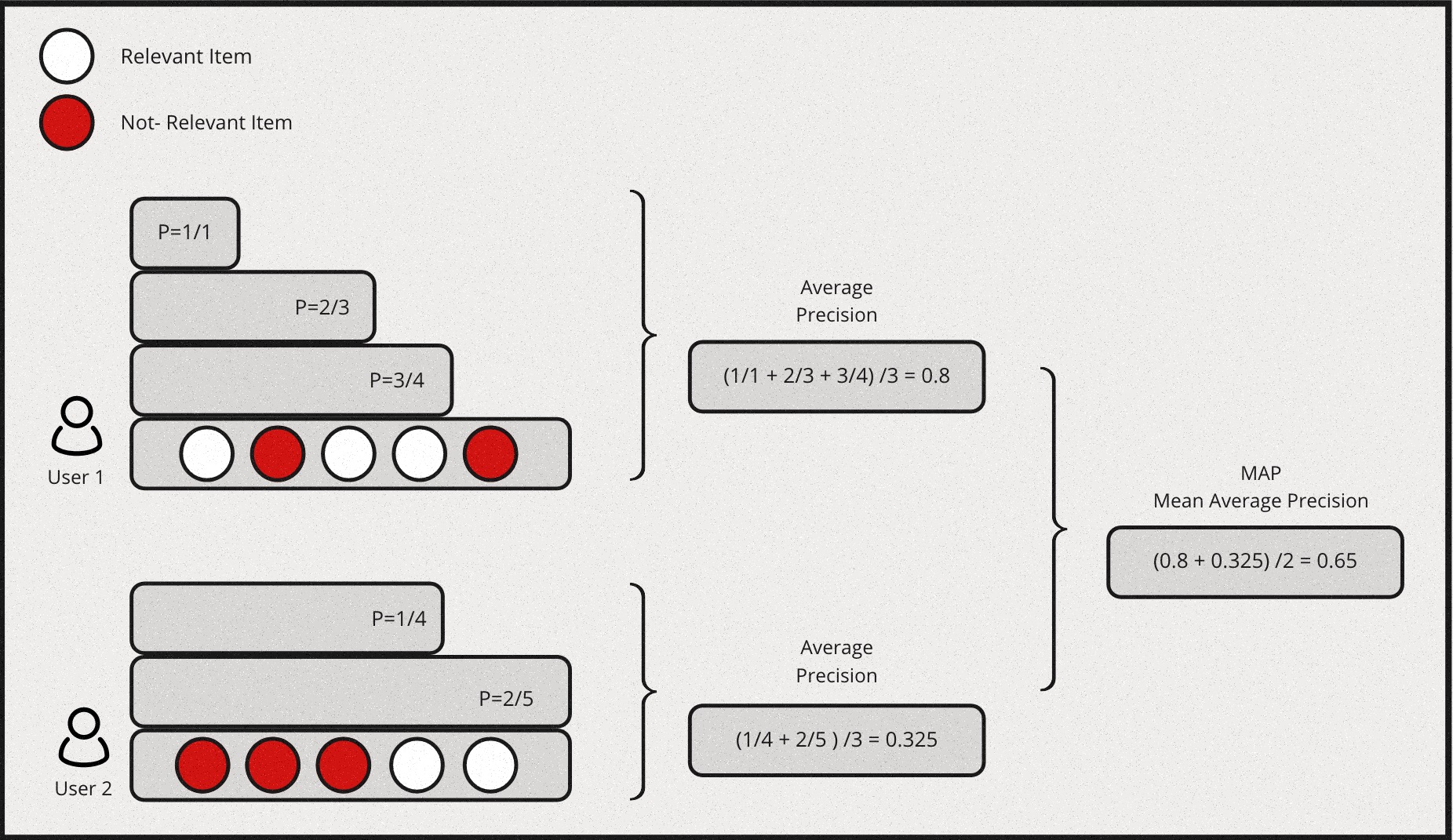
Mean Average Precision (MAP)

MAP is a measure based on binary label of relevancy. To compute this first we define precision at k for a given query \(P@k(q)\) as:

\[P@k(q) \equiv \frac{\sum_{i=1}^k r_i}{k}\]

for an ordered list of prediction \(r_i\) for all \(k\) items. \(ri=1\) if it is relevant and 0 otherwise.Then we define the average precision given a query \(AP(q)\) at \(k\) items as:

\[AP(q)@k \equiv \frac{1}{\sum_{i=1}^k r_i} \sum_{i=1}^k P@i(q) \times r_i\]

Mean Average Precision is just the mean of \(AP(q)\) for all queries:

\[MAP \equiv \frac{\sum_{q=1}^Q AP(q)}{Q}\]

Also, MAP is an order sensitive metric because of the term \(r_i\) in the calculation of AP. It is essentially taking the average of precision at each ranking position and penalizing the precision at positions with irrelevant item by strcitly setting them to zeroes.

Here is a simple example for computing MAP:

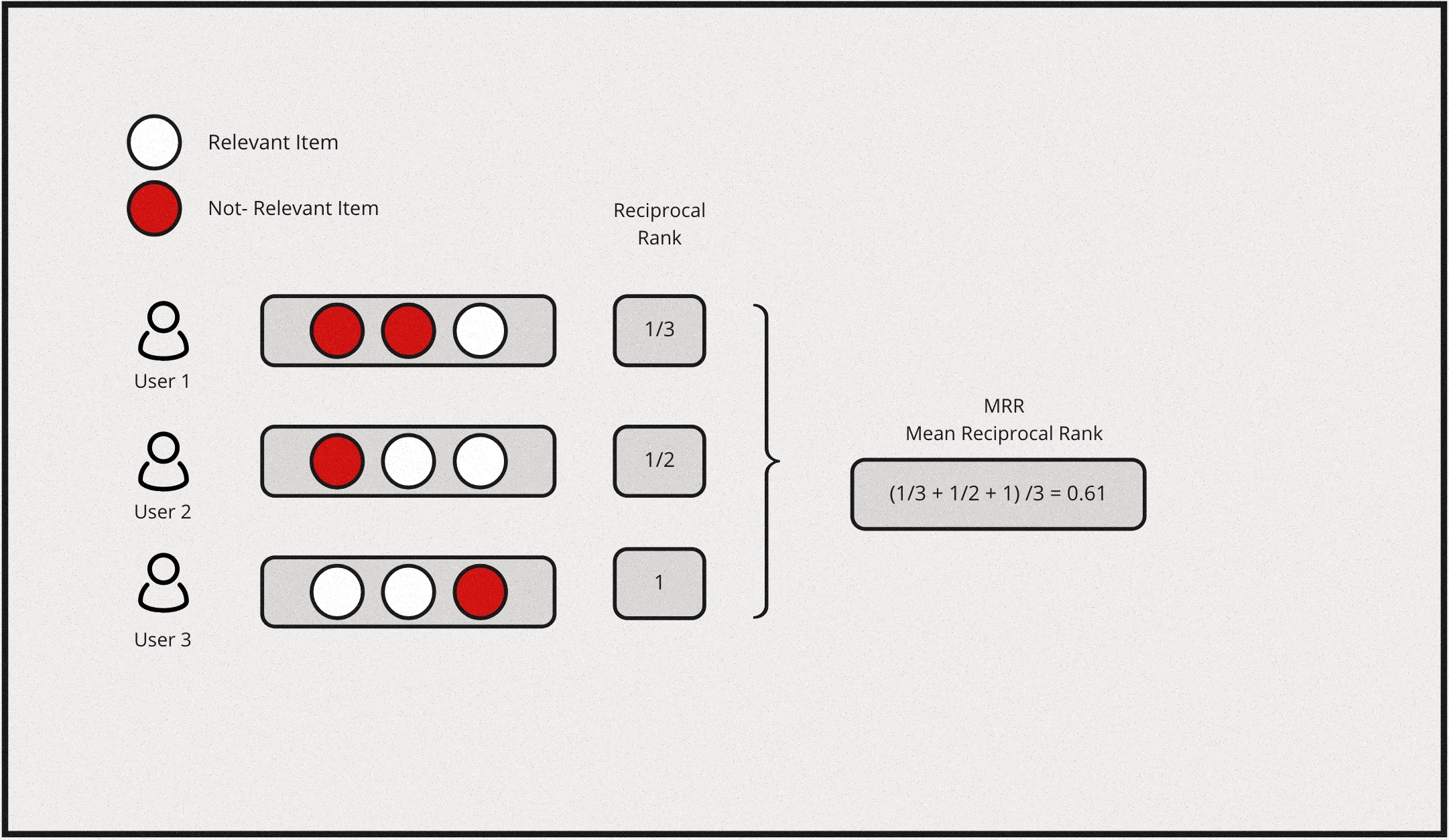
Mean Reciprocal Rank (MRR) & Expected Reciprocal Rank (ERR)

Reciprocal rank metrics focus mainly on the first correctly predicted relevant item in a list. Given a list of items, and say \(r_i\) is the rank of the highest ranking relevant item & if the the 2nd item is the first relevant item in the list, then the reciprocal rank for this query would be \(\frac{1}{2}\). By extension, each query will have a reciprocal rank. Hence, Mean reciprocal rank is essentially the average of reciprocal rank for all the queries, which would be represented as follows:

\[MRR \equiv \frac{1}{Q} \sum_{i=1}^Q\frac{1}{r_i}\]

Expected reciprocal rank tries to quantify how useful a document at rank \(i\) conditioned on the degree of relevance of documents at rank less than \(i\) are. The intution behind this is based on the empirical findings from web search task, that the likelihood a user will examine the document at rank \(i\) is dependent on how satisfied the user was with previously observed documents in the list.

Lets assume the probability of a user finding the result is satisfied at position \(i\) in a list of items is denoted as \(R_i\) & the likelihood of a session for which the user is satisfied and stops at position \(r\) is: \[\prod_{i=1}^{r-1}(1 - R_i)R_r\]

Now we can model \(R_i\) such that it is an increasing function of relevance:

\[R = R(g) \equiv \frac{2^g - 1}{2^{g_{max}}}\]

where \(g\) is the graded relevance such that \(g \in \{0, 1, ..., g_{max}\}\) & \(g = 0\) implies an irrelevant document and \(g = g_{max}\) implies a relevant document.

Now we can define ERR as follows:

\[ERR \equiv \sum_{r=1}^n\frac{1}{r}R_r\prod_{i=1}^{r-1}(1-R_i)\]

Here \(\frac{1}{r}\) is treated as a utility function \(\tau(r)\) that satisfies \(\tau(1) = 1\) and \(\tau(r) \rightarrow 0\) as \(r \rightarrow \infty\).

Note that ERR is a metric on a list with a single query, To evaluate results from multiple queries, we will need to further average ERRs among queries.

Here is a simple example for computing MRR:

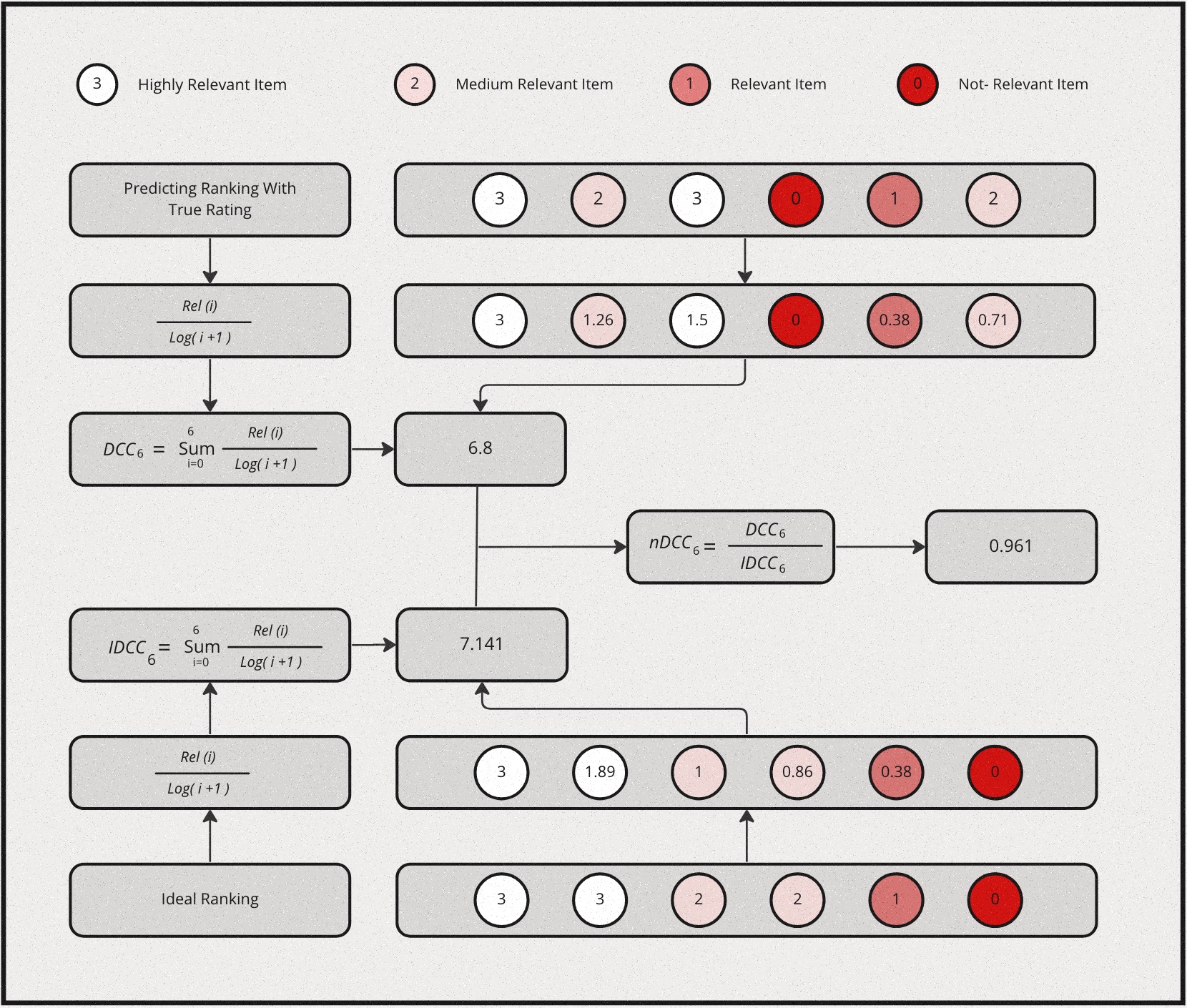
Normalized Discounted Cumulative Gain (NDCG)

Normalized Discounted Cumulative Gain (NDCG) is one of the most popular metric for measuring the quality of a set of ranked items in search or recommendations. If we were to break the assumptions made by this metric in simple terms, it would be as follows:

Cumulative Gain: Very relevant items are more useful than somewhat relevant items which are more useful than completely irrelevant items.
Discounting: Relevant items are more useful when they appear earlier in a list of ranked items.
Normalization: The ranking results should be irrelevant to the query performed.

Let’s define Discounted Cumulative Gain at position \(k\) as follows:

\[DCG@k \equiv \sum_{i=1}^k\frac{2^{l_i} - 1}{log_2(i + 1)}\]

where \(l_i\) is the grading of relevance at rank \(i\). Intutively, the numerator is simply an increasing function of relevance, the more relevant the higher. This is the gain from each item. The denominator is a decreasing function of ranking position, this is the discounted component of the metric. Collectively, higher relevance gains more score, but the lower it is ranked the higher also the discount. Essentially, the metric will prefer higher relevant item to be ranked higher, which is the desired outcome.

NDCG is then defined as:

\[NDCG@k = \frac{DCG@k}{IDCG@k}\]

where \(IDCG@k\) is the Ideal DCG@k given the result. DCG@k is calculated by sorting the given list of items by its true relevance labels. and IDCG@k is the maximum possible DCG@K value one can get given a ranked list of items.

Here is a simple example for computing NDCG:

Learning to rank with Multiple Objectives

MOO - The What, The Why & The How.

After that long detour, let’s now look into Multiple Objective Optimisation applied to Ranking problem within a marketplace setting involving multiple stakeholders. Let’s do so with a simple illustrative example that involves similar item recommendations. Specifically, let’s understand Why this is needed first.

Picture this, A User has browsed and explored a bunch of different red shirts they are planning to buy, and on one such open tab we’ve got a shirt that they are closely examining. Now, the recommendation system in the backend is also generating a bunch of similar shirts that they might be interested to explore. Let’s say the recommendation system is optimising for two different objectives - firstly, to show relevant and personalised shirts similar to their style based on interaction history. Secondly, the platform also wants to make sure it’s making a good profit on each sales that the recommendation system generates or leads to. Hence, they would also want to promote shirts with good porfit margin. How would we do this?

Let’s start by defining our objectives:

Objective I	Objective II
Personalisation	Price Margin

Let’s also say the item options available to us to be displayed (let’s focus on finding the top-1 item at the moment.) if plotted on a graph look something like this:

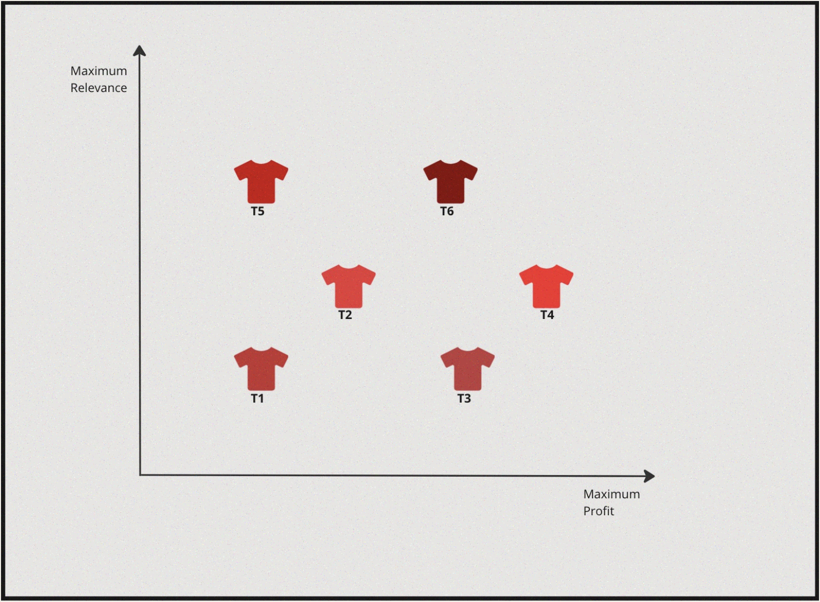
Now, essentially we want to maximise profit margin but also we want to maximise for highly personalised & relevant shirt. If we were to solve this from a lens of single objectve optimisation two scenarios would arise:

Case-I: Applying 1D Optimisation to objective I followed by optimising for objective II, i.e First we can find Highly Personalised shirts and then search for the shirt that also provides maximum margin.
Case-II: Applying 1D Optimisation to objective II followed by optimising for objective I, i.e First we can find High Profit margin shirts and then search for the ones which are also Highly Personalised & relevant for the user’s style.

For a simple and better understanding of the concept, assume that someone is trying to find the best red shirt from both the perspectives manually in a physical store, and let’s further also assume its a dark room.

Case I : Highly Personalised & High Profit margin

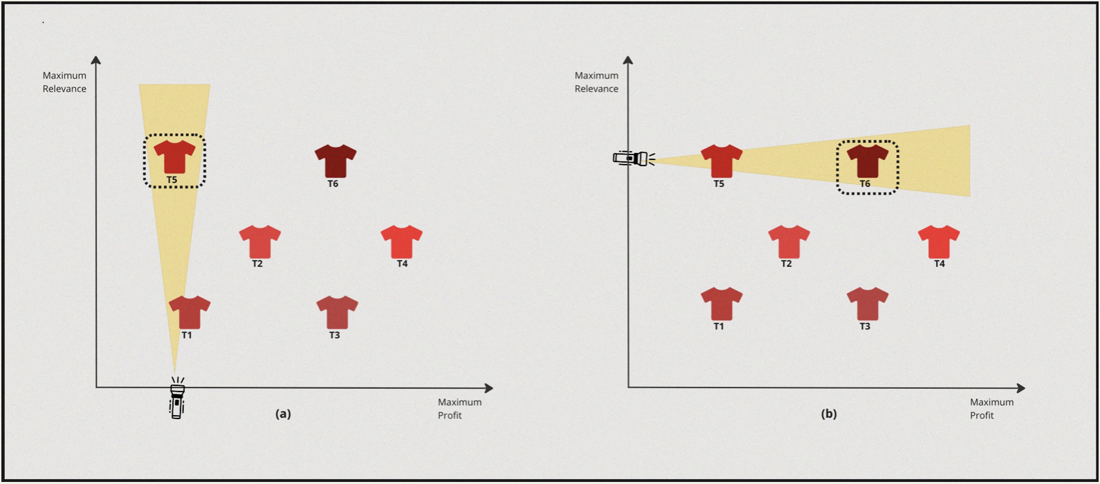
So, in this case the solver turns the torch on towards the relevance axis and discovers \(T5\) as the most suitable candidate.
Now from this point the solver turns towards the profit axis and turns the torch on and discovers \(T6\).

Case II : High Profit margin & High Personalisation

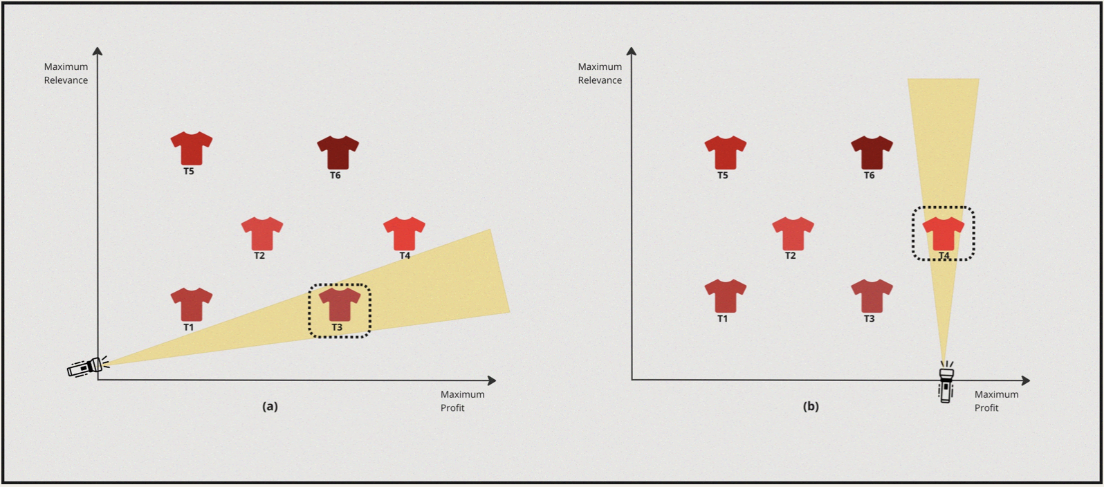
In this case the solver turns the torch on towards the profit axis and discovers \(T3\) as the best candidate.
Now from this point the solver turns towards the relevance axis and turns the torch on and discovers \(T4\).

What do we have as of now:

Process	1st Optimization Objective	2nd Optimization Objective	Optimal Solution
1	Personalisation	Profit Margin	\(T6\)
2	Profit Margin	Personalisation	\(T4\)

So, that seems odd. There are multiple solutions. Depending on what we want to achieve- If we want to optimize for both objectives and find the best solution, Going about in the above method is not the best way. Instead, we need to optimize to find solutions for both objectives collectively. The set of optimization methods that enables this is called Multiple Objective Optimization.

Let’s define what MOO is & try to understand some other key concepts associated with it.

Basic Concepts - Defining the MOO Problem, Pareto Optimum & Pareto Frontier

MOO: Optimization that involves identifying the values of decision (or free) variables that generate the maximum or minimum of one or more objectives. In most engineering problems, there may exist multiple, conflicting objectives and solving the optimization problems is not trivial or may not be even feasible sometimes. One way to formulate this is as follows:

Given \(m\) inequality constraints & \(p\) equality constraints identify a vector \(\bar{x}^*_n = [x^*_1, x^*_2,...,x^*_n]^T\) that optimizes

\[\bar{f}_k(\bar{x}_n) = [o_1(\bar{x}_n), o_2(\bar{x}_n),..., o_k(\bar{x}_n)]^T\]

such that

\[g_i(\bar{x}_n) ≥ 0, i = 1, 2, . . . , m\]

\[h_i( \bar{x}_n) = 0, i = 1, 2, . . . , p\]

where \(\bar{x}_n = [x_1, x_2, . . . , x_n]^T\) is a vector of \(n\) decision variables. The constraints determine the “feasible region” \(F\) and any point \(\bar{x}_n ∈ F\) gives a “feasible solution” where \(g_i( \bar{x}_n)\) and \(h_i( \bar{x}_n)\) are the constraints imposed on decision variables. The vector function \(\bar{f}_k(\bar{x}_n)\) above is a set of \(k\) objective functions, \(o_i(\bar{x}_n)\) for \(i = 1, · · · , k\), representing k non-commensurable criteria.

Pareto Optimum: A point \(\bar{x}^∗\) is “Pareto optimal” (for minimisation task) if the following holds for every \(\bar{x}_n ∈ F\)

\[\bar{f}_k(\bar{x}^*_n) ≤ \bar{f}_k( \bar{x}_n)\]

where \(\bar{f}_k(\bar{x}_n) = [o_1(\bar{x}_n), o_2(\bar{x}_n),..., o_k(\bar{x}_n)]^T\), \(\bar{f}^*_k(\bar{x}^*_n) = [o_1(\bar{x}^*_n), o_2(\bar{x}^*_n),..., o_k(\bar{x}^*_n)]^T\)

Pareto optimality gives a set of nondominated solutions. A feasible solution \(x\) is called “weakly nondominated” if there is no \(y ∈ F\) , such that \(o_i(y) < o_i(x)\) for all \(i = 1, 2, ..., k\). This means that there is no other feasible solution that can strictly dominate \(x\). A feasible solution \(x\) is called “strongly nondominated” if there is no \(y ∈ F\) , such that \(o_i(y) ≤ o_i(x)\) for all \(i = 1, 2, ...k\), and \(o_i(y) < o_i(x)\) for at least one \(i\). This means that there is no other feasible solution that can improve some objectives without worsening at least one other objective. If \(x\) is “strongly nondominated”, it is also “weakly nondominated”.

Pareto Frontier: A set (of feasible solutions) that is Pareto efficient is called the Pareto frontier, Pareto set, or Pareto front. The optimal solutions can be determined based on the tradeoffs within this set based on a designer’s decisions for acceptable performance.

Popular methods applied to LTR Setting.

Over the years, numerous approaches have been applied in LTR settings. Broadly most of these approaches can be classified into four categories as follows:

Label Aggregation
Constraint Optimization
Model Fusion/Aggregation
Lexicographic

Now, lets us define these approaches.

Label Aggregation

In this method, we combine all objective functions to form a single objective function which is then minimized. Once we convert the multi-objective into a single objective by combing the labels, we solved the given LTR problem as the single objective function. Let’s say for given query q, and products P, we have two different labels, \(ℓ_1(q,p)\) a similarity score between query and prodct, and \(ℓ_2(p)\) a profit margin for a product, we can put a new label as \(ℓ(q, p) = \alpha·ℓ_1(q, p) + (1 − \alpha)·ℓ2(p)\)

Note: Here \(\alpha\) is manually chosen by the user. If \(\alpha \in \{0,1\}\), the problem is reduced to a single objective optimization.

In general, given k objectives rank function looks like below:

Minimise,

\[f(x) = \sum_{i=1}^k{\alpha_i * f_i(x)}\]

Subject to \[\sum_{i=1}^k{\alpha_i = 1}\]

Advantages

It gives a clear interpretation of the multi-objective function and generalize it.
It allows multiple parameters to be set to reflect preferences.

Disadvantages

It tries to optimize for each objective function, which can be computationally expensive.
The setting of parameters \((\alpha_i)\) is not intuitively clear when only one solution point is desired.

Constraint Optimization

This method optimizes the single most important objective \(f_{primary}(x)\) and treat the other objectives as constraints with pre-determined upperbound. As we saw eariler, let’s say have two objectives to optimize. First objective is \(ℓ_1(q,p)\) - similarity score between \((p,q)\) and second \(ℓ_2(p)\) - profit margin for \(o\). Then we could consider \(ℓ_1(q,p)\) as primary objective and \(ℓ_2(p)\) as secondary objective. In this method we will optimize for primary objective \(ℓ_1(q,p)\) subject to \(ℓ_2(p) \lesssim \epsilon\).

In general, given k objectives the ranking function is as follows:

\[ \min_{\forall x_i} f_l(x)\]

Subject to \[ f_i(x) \lesssim \epsilon_i, \forall i \not = l ,\] \(\epsilon_i\) is upperbound for \(f_i(x)\). And, \(f_l(x)\) is the primary function to optimize.

Advantages

It focuses on a single objective with limits on others.
It always provides a weakly Pareto optimal point, assuming that the formulation gives a solution.
It is not necessary to normalize the objective functions.

Disadvantages

The optimization problem may be infeasible if the bounds on the objective functions are not appropriate.

Model Fusion/Aggregation

This method is an aggregation of multiple independent ranking models. The final ranking socre is obtained by a convex combination of multiple models. As we saw earlier if we have two objectives, let’s say \(ℓ_1(q,p)\) - similarity between query and product and \(ℓ_2(p)\) - profit margin. Then first we train the \(M_{l1}\) model which optimizes for similarity score between (q,p). And further we also independently train another model \(M_{l2}\) which optimizes for the profit margin. The linear combination of the models can be formulated as \(M(q,p) = \alpha·M_{l1}(q, p) + (1 − α)·M_{l2}(p)\), where the hyperparameter \(\alpha \in[0, .,., 1]\) controls the tradeoff between the two model scores.

In general, given k objectives the ranking function looks as follows:

\[M(x) = \sum_{i=1}^k (\alpha_i * M_i (x))\]

where, \(M_i(x)\) is an independently trained model for optimizing \(i^{th}\) objective.

Advantages

This is used as a post-rank method, and as such easy to tweak weighting parameters.
Learning for one single objective will not be affected by other objectives (decoupled objectives).

Disadvantages

It’s difficult to find the optimal weight for the final ranking.

Lexicographic

When we have more than one objective, we rank the items by ordering the objective functions according to their importance. As mentioned earlier, we have two objective functions, \(ℓ_1(q,p)\) similarity between query and product as pprimary objective and \(ℓ_2(p)\) profit margin as the secondary objective. Then We will order the items according to the primary objective \(ℓ_1(q,p)\) and if a tie happens, then we use \(ℓ_2(p)\) the secondary objective score to break the tie.

In general, given k objectives, the rank function looks like below:

Minimise,

\[ f_i(x)\]

Subject to \[ f_j(x) \lesssim f_j(x_j^*)\] \(j = 1\) to (\(i - 1\)) and \(i > 1\) ; \(i = 1\) to \(k\)

Here, we rank the function based on \(f_i\), and where a tie occurs we break the tie based on \(f_{(i+1)}\) score.

Advantages

It is a unique approach to specifying preferences.
It does not require that the objective functions be normalized.

Disadvantages

It requires that additional constraints be imposed.
It is computation heavy if we have more objectives.

Few Examples in the Wild

A Multi-Objective Learning to Re-Rank Approach to Optimize Online Marketplaces for Multiple Stakeholders.

Read the Original Paper over here: Original Paper

First, let’s look at an example from Expedia. Being a service provider they are trying to optimize for the following objectives:

Consumer’s Conversion Rate or Click Through Rate.
Maximum transaction commission from the supplier.

A supplier pays a marginal amount of the sales transaction as a commission to the platform. Let’s say the product’s cost is \(c\) and the selling price is \(p\) then the margin is \(m = p-c\).

To achieve the above objectives, the optimization function is defined as follows:

\[\max_{\alpha, \beta}L(m|u) = \sum_{i=1}^n \log(u_i) + \alpha \log(p_i) + \beta \log(\frac{m_i}{p_i})\]

where \(\alpha\) and \(\beta\) are tuning parameters.

\(\log(u_i)\) = User possibility to do transaction.

\(\log(p_i)\) = supplier interest for selling the product at price \(p\).

\(\log(m/p)\) = profit margin define as percentage here.

In these objective functions, we have contradictory relations with suppliers and consumers by nature. On the other side, service providers want higher commission benefits from suppliers at an indirect cost to consumers. For such problems, there is no unique Pareto optimal solution because of the complex and opposing interactions of the different stakeholder interests.

Here they give priority to promoting items to higher positions that better satisfy a transaction commission objective while staying as close as possible to the original ranking. The new ranking score function looks like the below:

\[ \forall_u \in u, u^{′} = u + \alpha\log(p) + \beta(x,m)\log(\frac{m}{p})\]

To reduce the distance between the new vs old score vectors, they use the Kendall tau correlation measure. The updated objective function looks like the below:

\[\min_{\alpha, \beta}L(m|u, X) = L_r(\frac{m}{X}) + \gamma(1 - K^{'}(u, u^{′})) \]

Here, \(K^{'}(u, u^{'})\) is playing the role of a similarity-based regularizer with the original ranking order u being the reference point to the new ranking order \(u^{′}\). The hyperparameter \(\gamma\) gives the balance between our objective function.

To evaluate the LTR method, they use an in-house Expedia dataset built from worldwide hotel searches collected during 2016. The new ranking methods give a lift of +16.7% on the NDCG of margin, but at the same time, this incurs a decrease of -5.9% in terms of the NDCG of customer preferences.

The paper also uses the following formula to calculate the risk and reward to further evaluate the new objective function:

\[ Risk = \frac{1}{|q|} \sum_q NDCG@10(LRR) < NDCG@10(Baseline)\]

\[ Reward = \frac{1}{|q|} \sum_q NDCG@10(LRR) > NDCG@10(Baseline)\]

They have found that the risk is lower than the baseline and the reward much higher.

This experiment shows that multi-objective is always a trade-off between the two objectives: Conversion rate vs Margin. They would like to further test with real-world performance via \(A/B\) testing.

Joint Optimization of Profit and Relevance for Recommendation Systems in E-commerce

Read the Original Paper over here: Original Paper

Traditionally, e-commerce-based recommendation systems focus on optimizing for relevance by predicting the purchase or click probability of an item. The relevance-centric approach is capable to increased the conversion rate but does not guarantee a maximum profit for either a platform or seller. In this paper from Etsy, where they discussed a novel revenue model, which optimizes for two objectives:

Maximising the Revenue
The probability of the purchase.

To maximize the likelihood, the objective function is defined as follows:

\[\max_{w \in R^n, b \in R} l(w,b) := - \sum_{i=1}^{m} \log(1 + exp(-y_i(w^T x_i + b)))\]

Here, \(x_i\) = \(i^{th}\) training sample \(x_i \in R^n\) \(y_i\) = label whether a recommended item is purchased or not

Let’s say \(\pi_i\) is the price of item, then the objective function for maximizing profit is as below:

\[ρ(w,b) := \sum_{i=1}^{m} E[\pi_i, y_i] = \sum_{i=1}^{m} \pi_i (2prob[y_i = 1|x_i;w] - 1)\]

\[= \sum_{i=1}^{m} 2\pi_i\sigma(w^T x_i + b) - \pi_i,\]

The combined objective function will be:

\[\max_{w\in R^n, b\in R } l(w,b) + \mu ρ(w,b)\]

To optimise the above objective, \((w,b)\) parameters need to be found which can fit \(l(w,b)\) to maximise the likelihood while maximizing the expected revenue (via \(ρ(w, b)\)). Here, \(\mu ≥ 0\) is a hyperparameter of the model that controls the tradeoff between the two objectives. Once the optimal parameters are learned, they use them to rank a set of candidate items.

They have used the following metrics to evaluate the performance of the proposed model

Profit@K: profit generate by kth highest ranked item
Average price: Average price of the k highest ranked item
AUC: to measure relevance
NDCG@5

Etsy has done an offline evaluation of the proposed model. They found the proposed revenue model attains the highest AUC and profit@k for all K values. Note they used K value up to 3. They observe that the revenue model has a 3.57% increase in AUC and 9.50% in profit@1 compared to the baseline model. Also increases P-NDCG@k and AP@k for all k by at least 3.57% and 23.08% However, the proposed model results in a 10.76% and 16.06% decrease in AUC compared to the baseline.

The overall revenue model can increase profit for the platform while retaining high relevancy for users. They would like to assess revenue model performance in the face of real user traffic via an online A/B experiment.

Using Bayesian optimization for balancing metrics in recommendation systems

Read the Original article over here: Original Article

Let’s now look into an article from Linkedin where they describe their approach towards building their notifications recommendation system, which notifies members about various activities within their network. To build an efficient notification system, they are optimizing for the following objects:

CTR
Number of sessions (i.e the user visits & app open rate)

The CTR and session objectives can be conflicting, because sending more notifications to members may lead them to visit an app frequently. And It increases the overall number of sessions but on the other side, it can decrease CTR because of the quality of the notification.

The overall objective function they define is as follows:

\[p_{click} + \alpha * \Delta p_{visit} > \gamma\]

where,

\(p_{click}\) is the probability of click by member
\(\Delta p_{visit}\) can be defined as \(p(\frac{visit}{sent})\) - \(p(\frac{visit}{not sent})\). Which is basically the difference between sending a notification now vs not sending a notification.
\(\alpha\) is the hyperparameter that measures the relative importance of the two utilities.
\(\gamma\) is the threshold applied.

Finding an optimal value of \(x=\{\alpha,\gamma\}\) can maximize the sessions without compromising on CTR and send volume. To ensure the overall performance, they used \(c1\) and \(c2\) constraints as contained for CTR(x), and Send Volume(x).

The updated objective function looks like the below:

\[ \max_{\forall x_i} , f_{session}(x)\]

Such that, \[f_{CTR}(x) > c_1, f_{sentVolume} (x) < c_2\]

Using the above constraints, they define a single objective function as below:

\[\max_x f(x) = f_{session}(x) + \lambda(1 \{f_{CTR}(x) > c_1 \} + 1\{f_{sentVolume(x)} < c_2\}),\]

By converting a MOO into SOO using constrained-based optimization, they learn global hyperparameters (i.e., a single value) for all members. Further, they evaluate and improve upon this via online A/B experiments.

Conclusion

In this rather long post, we looked into common design patterns for building modern recommendation systems, Common styles of training ranking models & Popular metrics for evaluating these systems and also looked at the task of multiple objective optimizations and their application within Learning to rank. We also looked at a few examples of multi-objective ranking from the industry - and one common trend that we observed is that simple techniques like label aggregation, model aggregation, or constrained optimization work surprisingly well in practice.

With that said, In the upcoming blogs, we’ll do a deep dive into each of these approaches and look at how one could implement these in practice with an open-source dataset.

For any suggestions/feedback or improvements to this article - or maybe just for a casual chat feel free to reach out to us: Bharath G.S & Rita Anjana & if you found this article useful - Please share it with others and let us know!

Also, If you prefer to read this as a PDF - download it over here: article-pdf

Acknowledgement

Thanks to Jordan Hochenbaum for reading drafts of this and providing valuable feedback.

The Path towards Marketplace recommendations: Part-I

The Backdrop

Introduction

Stakeholders, Objectives & the Objective interplay

A Quick Recap on modern recsys

Candidate retrieval

Ranking

A Quick Recap on Learning to Rank

Ranking Task

Pointwise method

Pairwise method

Listwise method

A Quick Recap on Ranking Evaluation metrics

Mean Average Precision (MAP)

Mean Reciprocal Rank (MRR) & Expected Reciprocal Rank (ERR)

Normalized Discounted Cumulative Gain (NDCG)

Learning to rank with Multiple Objectives

MOO - The What, The Why & The How.

Case I : Highly Personalised & High Profit margin

Case II : High Profit margin & High Personalisation

Popular methods applied to LTR Setting.

Label Aggregation

Advantages

Disadvantages

Constraint Optimization

Advantages

Disadvantages

Model Fusion/Aggregation

Advantages

Disadvantages

Lexicographic

Advantages

Disadvantages

Few Examples in the Wild

A Multi-Objective Learning to Re-Rank Approach to Optimize Online Marketplaces for Multiple Stakeholders.

Joint Optimization of Profit and Relevance for Recommendation Systems in E-commerce

Using Bayesian optimization for balancing metrics in recommendation systems

Conclusion

Acknowledgement

Reference